Window Functions in Postgres for Ranking and Running Totals

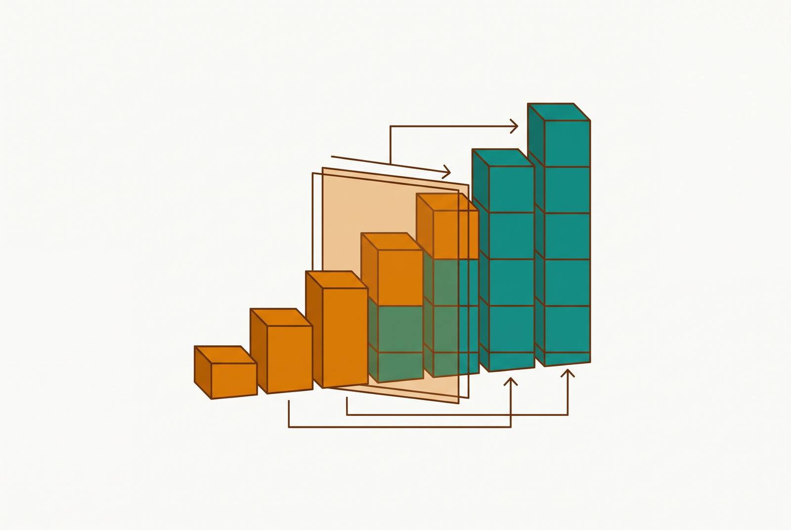
Window functions solve a problem that used to make grown developers write self-joins at 11pm: how do you rank rows, or add up a running total, without collapsing your result set down to one row per group? A GROUP BY smashes everything into a summary. A window function does the math and hands every row back to you, untouched, with the answer sitting right next to it. That's the whole trick, and once it clicks, a lot of SQL that used to feel like a puzzle becomes a two-line query.

Before window functions were widely supported, getting a running total meant a correlated subquery that re-scanned the table for every single row, or a self-join that multiplied your row count and your headache in equal measure. Window functions replace all of that with one pass over the data. Postgres also happens to have one of the more complete implementations of the SQL standard here, including frame options (GROUPS, EXCLUDE) that other major databases didn't support until later.

Window functions run after GROUP BY and after regular aggregates are computed. That ordering matters, and it's also why you can use a window function in SELECT or ORDER BY, but never in WHERE, JOIN, or GROUP BY itself. The database hasn't finished figuring out your window results by the time it's evaluating those clauses. Keep that one rule in your back pocket. It explains half the "why won't this filter work" questions that come up later.

This guide sticks to Postgres syntax. The concepts (partitioning, ordering, framing) apply almost everywhere window functions exist, including SQLite (3.25+), MySQL (8.0+), SQL Server, and Oracle. But a few of the sharper tools here, like GROUPS framing, frame exclusion, and FILTER, are Postgres-specific or gated behind certain versions. Copying a query into a different engine can break it for this reason.

The anatomy of the OVER() clause: PARTITION BY, ORDER BY, and the frame

Every window function follows the same shape:

SELECT col, window_function(col) OVER (
  PARTITION BY partition_col
  ORDER BY order_col
  frame_clause
)
FROM table;

Three parts, each doing a different job.

PARTITION BY splits your rows into logical groups, the same way GROUP BY would, except nothing gets collapsed. Every row stays visible. If you leave it out, the function treats the whole result set as one giant partition.

ORDER BY inside OVER() decides the sequence rows are processed in in within each partition. For ranking and running totals, this isn't optional; it's the whole point. For a straightforward aggregate over an entire partition (say, total sales per region with no running component), you can skip it.

The frame clause is where most people trip up. It defines which rows, relative to the current row, the function actually looks at. Get this wrong and your running total or moving average will quietly produce the wrong number, no error, no warning, just a subtly broken report someone finds three weeks later.

Postgres gives you three frame modes:

ROWS: counts physical rows. "2 rows before this one" means exactly that, regardless of what the values are. RANGE: counts based on the value of the ORDER BY column. Rows that tie on that value are treated as peers and grouped together. GROUPS (Postgres 11+): counts distinct groups of equal ORDER BY values, rather than individual rows.

When you add an ORDER BY inside OVER() but don't specify a frame, Postgres defaults to RANGE UNBOUNDED PRECEDING, which is shorthand for RANGE BETWEEN UNBOUNDED PRECEDING AND CURRENT ROW. That default is exactly why running totals sometimes behave strangely on tied values, more on that in a bit.

UNBOUNDED PRECEDING and UNBOUNDED FOLLOWING just mean "start of the partition" and "end of the partition." And an empty OVER(), no partition, no order, means the function is looking at every row in the result set as a single window.

Two more tools to know about are FILTER, which lets an aggregate window function apply a condition before it ever sees a row (only rows passing the filter get counted), and EXCLUDE (Postgres 14+), which lets you remove specific rows, like the current row or its ties, from an otherwise normal frame.

Ranking functions: ROW_NUMBER, RANK, DENSE_RANK, and NTILE

Four functions, all answering some version of "where does this row rank within its group?" None of them need a frame clause. The differences come down to how they handle ties.

ROW_NUMBER() hands out a unique number to every row, starting at 1, no gaps, no ties, ever. Even if two rows have identical values on the ORDER BY column, they still get different numbers. This is the function to reach for when you need exactly N rows per group, no matter what the underlying data looks like.

RANK() gives tied rows the same rank, then skips ahead. Two rows tied for 2nd means the next row is ranked 4th, not 3rd. This mirrors how a leaderboard usually works: "tied for second" is a real, meaningful state, and the gap communicates that two people share the spot.

DENSE_RANK() also gives tied rows the same rank, but doesn't skip. Two rows tied at 2 means the next rank is 3. Good for tier-based labels, bronze/silver/gold, where you want continuous, gapless categories.

NTILE(n) does something different entirely: it divides rows into n roughly equal buckets, numbered 1 through n. Think quartiles or deciles. It's less about "rank" and more about "which segment does this row fall into."

Picture ranking products by units sold within each category:

SELECT product, category, units_sold,
  RANK() OVER (PARTITION BY category ORDER BY units_sold DESC) AS category_rank
FROM sales;

Each category resets its own ranking sequence. Bestsellers in electronics don't compete against bestsellers in home goods.

Running all three functions side by side on the same data makes the difference obvious immediately: same input, three different outputs, purely because of how each one treats ties. That's the whole decision tree in one table. Need unique positions? ROW_NUMBER. Want gaps to signal ties? RANK. Want gapless tiers? DENSE_RANK. Segmenting into buckets? NTILE.

Top-N per group: the CTE pattern that filters on window results

Remember the rule from earlier: window functions can't be filtered in the same SELECT's WHERE clause. So how do you actually get "top 3 products per category" out of the database?

Wrap it in a CTE:

WITH ranked AS (
  SELECT product, category, units_sold,
    ROW_NUMBER() OVER (PARTITION BY category ORDER BY units_sold DESC) AS rn
  FROM sales
)
SELECT * FROM ranked WHERE rn <= 3;

The window function does its work in the CTE. The outer query filters on the result of that work, which is now just a regular column.

Why ROW_NUMBER() instead of RANK() here? Because RANK() can hand you more rows than you asked for. If two products tie for 3rd place in a category, RANK() gives both of them a rank of 3, and your WHERE rn <= 3 filter lets both through, making it 4 rows instead of 3. ROW_NUMBER() guarantees exactly N rows per group, ties or no ties. Same pattern, swap rn <= 3 for rn = 1, gets you the single best row per group. Most recent order per customer. Highest sale per region. Same shape every time.

If a window function result shows up more than once in a query, say, once in SELECT and again inside a CASE expression, don't just repeat the OVER() clause. Wrap the calculation in a CTE and reference the column once it exists. Whether Postgres deduplicates identical window calls under the hood is not guaranteed, so don't rely on it doing that work for you.

Running totals with SUM() OVER and the frame clause that controls them

The basic building block:

SUM(amount) OVER (ORDER BY sale_date)

Because there's an ORDER BY, the default frame kicks in: RANGE UNBOUNDED PRECEDING. That gives a running, cumulative total, row by row, as sale_date increases.

Except there's a catch, and it's the same tie problem from before, occurring in a new place. RANGE RANGE treats rows with equal ORDER BY values as peers, so they all get the same running total, the total as of that date, not a row-by-row buildup. Two sales, both dated 2026-01-01, one from the North region and one from the South, both showing a running total of 3500.00, because RANGE lumped them together as one peer group.

If that's not the behavior you want, and often it isn't, switch to ROWS:

SUM(amount) OVER (ORDER BY sale_date ROWS BETWEEN UNBOUNDED PRECEDING AND CURRENT ROW)

Now the frame counts physical rows, not tied values. Same two January 1st sales now accumulate independently: 1500.00, then 3500.00. Each row gets its own step in the staircase, regardless of what date it shares with its neighbor.

Adding PARTITION BY region (or salesperson, or whatever grouping makes sense) resets the running total at each partition boundary, giving you a clean, independent cumulative sum per group instead of one long total across everything.

Percent of total is a variation on the same idea, and it doesn't need a frame clause at all:

100.0 * amount / SUM(amount) OVER ()

Swapping OVER() for OVER (PARTITION BY region) gives you percent of total within each region instead of across the whole dataset.

Cumulative min and max follow the same ROWS BETWEEN UNBOUNDED PRECEDING AND CURRENT ROW pattern, MIN(closing_price) OVER w, MAX(closing_price) OVER w, which is exactly what you'd use to track a stock's all-time low or high, updated as of each row, per ticker.

Moving averages and time-based rolling windows

A fixed-row moving average uses ROWS to define a sliding window of a set size:

AVG(amount) OVER (ORDER BY sale_date ROWS BETWEEN 2 PRECEDING AND CURRENT ROW)

That's a 3-row window, the current row plus the two before it. Simple, as long as the underlying data has one row per date. If it doesn't, if there are multiple sales per day, this window is counting rows, not days, and your "3-day average" quietly becomes something else entirely. The fix is to aggregate into daily totals in a CTE first, then run the moving average on top of that clean, one-row-per-day result.

When the window needs to be defined by actual time distance rather than a row count, that's where RANGE earns its keep:

SUM(amount) OVER (
  PARTITION BY salesperson
  ORDER BY sale_date
  RANGE BETWEEN INTERVAL '7 days' PRECEDING AND CURRENT ROW
)

This gives a rolling 7-day total. Doesn't matter if there are 2 rows or 20 rows in that span, the boundary is defined by the interval.

Rule of thumb: use ROWS when you want a fixed count of rows in the window. Use RANGE when the window should be defined by a value distance, like calendar days, no matter how many rows happen to fall inside it.

Frames don't have to look backward, either. This one looks forward:

AVG(temperature) OVER (
  PARTITION BY city
  ORDER BY date DESC
  ROWS BETWEEN CURRENT ROW AND 2 FOLLOWING
)

Frame boundaries can point in either direction from the current row. Nothing forces a window to only look at the past.

LAG and LEAD for period-over-period comparisons

LAG and LEAD grab a value from a nearby row without needing a self-join.

LAG(column, offset) reaches backward. Default offset is 1 row back. If there's no prior row (say, it's the very first row in the partition), it returns NULL.

LEAD(column, offset) does the same thing, forward.

Day-over-day change becomes a one-liner:

amount - LAG(amount, 1) OVER (ORDER BY sale_date) AS change

No self-join, no subquery, just a straight subtraction against the previous row's value. Percentage change takes a bit more, either calling LAG twice in the same query or, cleaner, computing it once in a CTE and referencing that.

Adding a partition makes LAG respect group boundaries:

LAG(amount, 1) OVER (PARTITION BY salesperson ORDER BY sale_date)

Now each salesperson's first row correctly returns NULL, instead of accidentally pulling in the last sale from a completely different person. That partition boundary is doing real work here, not just cosmetic grouping.

LAG also takes a third argument for a default value, which is returned instead of NULL when there aren't enough prior rows to look at. Small detail, but it saves a COALESCE down the line.

Between the two, this covers a wide range of comparison logic: month-over-month trend, drop-off analysis, or comparing this month to the same month last year (set the offset to 12 on monthly data).

FIRST_VALUE, LAST_VALUE, and NTH_VALUE, and why the frame clause matters for them

FIRST_VALUE(col) OVER (PARTITION BY x ORDER BY y) grabs the first value in the frame. With the default frame, this generally works exactly the way it sounds like it should, because the frame always includes the first row of the partition.

LAST_VALUE is where the default frame quietly betrays you. Remember, the default frame (RANGE UNBOUNDED PRECEDING to CURRENT ROW) only extends up through the current row, never past it. So LAST_VALUE under the default frame doesn't return the partition's actual last value, because the frame only extends up through the current row and never sees what comes after it.

The fix is to say so explicitly:

LAST_VALUE(col) OVER (
  PARTITION BY x ORDER BY y
  ROWS BETWEEN UNBOUNDED PRECEDING AND UNBOUNDED FOLLOWING
)

Now the frame actually spans the whole partition, and LAST_VALUE returns what you'd expect.

NTH_VALUE(col, 2) has the identical problem. Without extending the frame, it can produce unhelpful results when the desired row lies outside the current frame's reach. Same fix applies.

Postgres's own documentation warns that LAST_VALUE and NTH_VALUE produce unhelpful results under the default frame. Relying on the default here is risky, and an explicit frame clause spanning the full partition is the safer approach.

Named windows with the WINDOW clause

Repeating the same PARTITION BY / ORDER BY / frame combination across four different function calls in one query gets tedious, and worse, error-prone if you need to change it later and miss one. The WINDOW clause solves that:

SELECT
  salesperson,
  sale_date,
  amount,
  SUM(amount) OVER regional_window,
  AVG(amount) OVER regional_window,
  ROW_NUMBER() OVER regional_window
FROM sales
WINDOW regional_window AS (
  PARTITION BY region ORDER BY sale_date
  ROWS BETWEEN UNBOUNDED PRECEDING AND CURRENT ROW
)
ORDER BY sale_date;

Define the window once, right after FROM/WHERE and before ORDER BY, then reference it by name in every function call that needs it. Changing the definition once updates every function using it automatically. It also gives the query planner a clearer signal that these calls share the same sort requirement, which can help it avoid redundant work.

This isn't universal syntax. Postgres supports it, MySQL 8+ supports it, BigQuery supports it. Not every SQL dialect does, so don't assume it'll port cleanly.

Statistical and distribution functions: PERCENT_RANK, CUME_DIST, and NTILE

Three more tools, this time for describing where a row sits within a distribution rather than just its rank.

PERCENT_RANK() returns a value between 0 and 1, representing the row's relative position. Rows in the same peer group (tied values) get the identical PERCENT_RANK.

CUME_DIST() gives the cumulative distribution, the fraction of rows with an ORDER BY value less than or equal to the current row's. Always somewhere just above 0, up to 1.

NTILE(n) NTILE(n) functions here again, this time as a distribution tool rather than a ranking tool. NTILE(4) for quartiles, NTILE(10) for deciles, NTILE(100) for percentile buckets. Useful for behavioral segmentation: which spending decile does this customer fall into, which percentile does this transaction size land in.

PERCENT_RANK and CUME_DIST return a continuous score, a number that describes relative standing. NTILE returns a discrete label, a bucket number. Need a precise score? Reach for the first two. Need to sort people into groups? NTILE is the tool.

Performance considerations engineers should understand

The core performance case for window functions comes down to one thing: a single pass over the table. Postgres computes window function results in one scan. The self-join or correlated-subquery approach that window functions replaced required multiple passes over the same data, and each additional pass costs I/O and memory. That difference compounds fast as table size grows.

Postgres has continued improving window function execution across recent major versions, part of a broader, ongoing effort to make analytical SQL patterns cheaper to run at scale, though the exact gains depend heavily on the query shape, data volume, and version in question, so treat any specific benchmark as a starting point for testing against actual workload, not a guarantee.

Anyone writing these queries should think about partition size, index support on the ORDER BY columns, and whether a ROWS frame (usually cheaper to compute) will do the job instead of RANGE. Window functions are fast because they avoid redundant scanning, but that advantage still depends on the query being shaped sensibly for the data underneath it.