Full-Text Search in Postgres Without Elasticsearch

Postgres can search text without any outside help. That's the whole point of this piece: tsvector, tsquery, GIN indexes, ranking, even typo tolerance, all built in, all free, all sitting in a database most teams already run. Before getting into how that works, it helps to see exactly where the obvious approach, LIKE and ILIKE, falls apart.

Three specific ways, actually.

First, leading wildcards kill performance. A query like WHERE title LIKE '%shoes%' can't use a standard B-tree index, because the database has no way to know where in the string "shoes" might start. So it reads every row, every time. (There's a workaround using pg_trgm's GIN indexes, which handle leading wildcards fine, but plain LIKE doesn't get that benefit on its own.) On a table with a few hundred rows, nobody notices. On a table with ten million, that query is the reason the page spins.

Second, LIKE has no idea what words mean. Search for "running shoes" and it won't find "run shoe" or "runner's sneakers," because as far as LIKE is concerned, those are just different sequences of characters. There's no concept of a word having variants. It's matching letters, not meaning.

Third, there's no sense of relevance. A document with "shoes" in the title and a document with "shoes" mentioned once in paragraph twelve come back exactly the same. LIKE either finds a match or it doesn't. It can't tell you which match matters more.

This holds for the whole LIKE/ILIKE/~/~* family, including in current Postgres releases like version 18. These aren't rare edge cases that only show up on unusual data. They're structural limits. The operators were never built for search, they were built for pattern matching, and pattern matching is a much smaller job.

Meanwhile, think about what a real user actually types into a search box: "reccommended headphones noise canceling." Misspelled. No quotes. No operators. No boolean logic. Just words, typed the way people type when they're in a hurry. Users expect the system to be smart about that. LIKE has no mechanism to bridge the gap between what someone typed and what they meant.

Postgres has had an answer to all three of these problems for a long time. The question isn't whether the capability exists. It's whether the team building the app knows it's there.

How Postgres represents text for search: tsvector and tsquery

Full-text search in Postgres runs on two purpose-built data types, and understanding what each one does is most of the battle.

tsvector is what a document looks like after it's been prepped for search. Instead of storing a big blob of raw text, Postgres breaks it down into a sorted list of distinct root words (called lexemes), often with position information attached, so it knows where each word originally sat in the text.

tsquery is the same idea applied to a search request. It's a structured version of what someone is looking for, and it can express real logic: this word AND that word, this word but NOT that one, these two words next to each other.

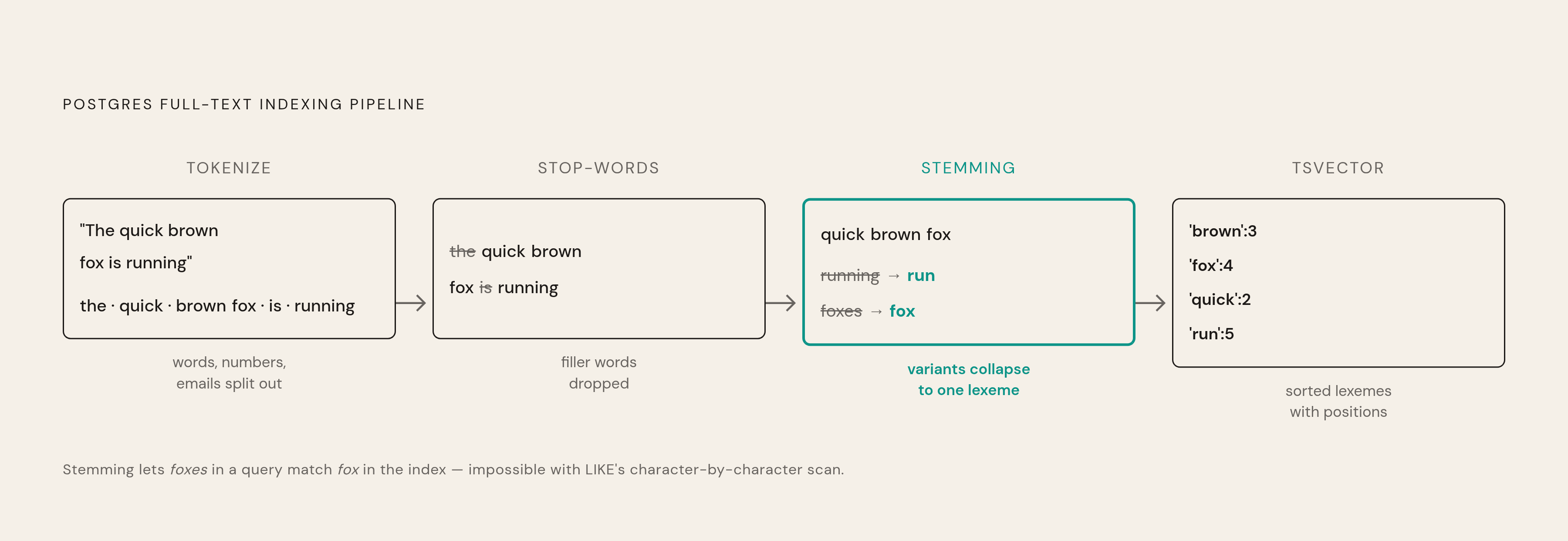
Getting from raw text to a tsvector involves a few steps, and they're worth walking through because they explain why the search feels "smart":

Tokenization: the raw text gets split into pieces, words, numbers, email addresses, whatever tokens exist. Stop-word removal: common filler words like "the," "and," "is" get dropped. They add noise, not meaning. Stemming: "running," "runs," and "ran" all collapse down to one lexeme, "run." Search for any variant, match all of them.

What comes out the other end is compact and ready to be indexed and searched fast.

The actual matching happens through the @@ operator. It asks a simple question: does this tsvector satisfy this tsquery? That's a fundamentally different operation than comparing characters one by one, the way LIKE does. It's matching processed meaning, not raw text.

A quick example makes this concrete:

to_tsvector('english', 'The quick brown foxes jumped')

produces something like 'brown':3 'fox':4 'jump':5 'quick':2. Notice "foxes" became "fox," "jumped" became "jump," and "The" disappeared entirely as a stop word.

And:

to_tsquery('english', 'quick & foxes')

produces 'quick' & 'fox'. Same stemming applied to the query side, so "foxes" in the search and "fox" in the document line up.

GIN indexes: the data structure that makes FTS fast at scale

None of the above is fast on its own. Speed comes from how it's indexed, and that's where GIN comes in. GIN stands for Generalized Inverted Index, and the concept is the same one behind the index at the back of a textbook: instead of scanning every page for a word, look the word up, and the index tells directly which pages have it.

A GIN index for full-text search maps every unique lexeme to the list of rows that contain it. Search for "run," and Postgres goes straight to the rows tagged with "run," instead of reading the whole table to check.

That distinction matters more as data grows. Lookup time with a GIN index depends on how many rows actually match, not on how many rows exist in the table overall. A sequential LIKE scan gets slower as the table grows, in a straight line, forever. A GIN-indexed FTS query stays fast, because it was never reading the whole table to begin with.

GIN indexes are slower to build and slower to update than a standard B-tree index. Every insert or update has more index bookkeeping to do. But for read-heavy workloads on large amounts of text, the query-time payoff is dramatic enough that the tradeoff is easy to accept. Different index types exist for different jobs. GIN is the one built for this job.

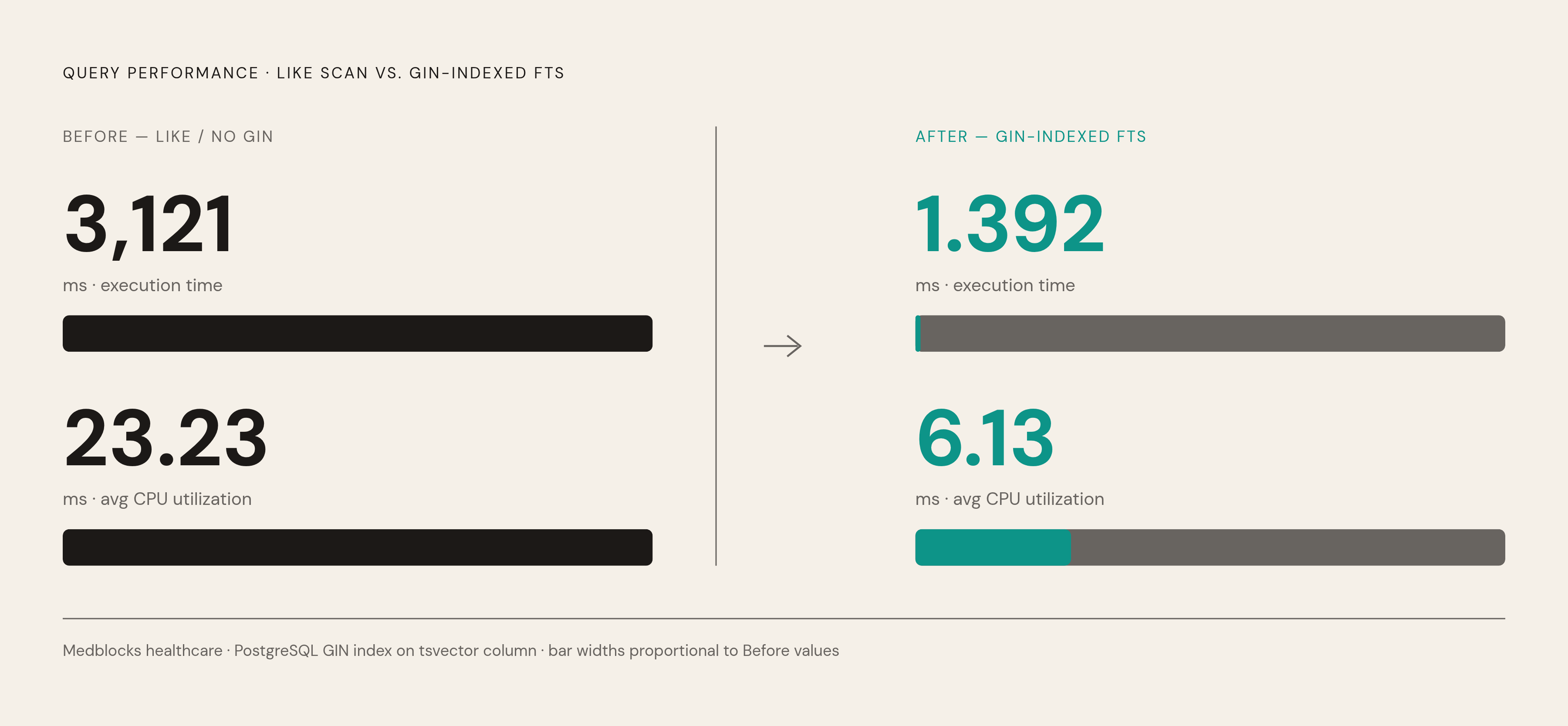
What does that payoff look like in practice? One healthcare team, Medblocks, switched patient search over to Postgres FTS backed by a GIN index and cut execution time from 3,121ms to 1.392ms. Average CPU utilization on those queries dropped from 23.23ms to 6.13ms. That's not a marginal tuning win. That's the difference between a feature that feels broken and one that feels instant.

Setting up FTS correctly: stored tsvector columns, generated columns, and triggers

Building a tsvector is only useful if it stays current. There are three ways to keep a search column in sync, and they get more automated as the list goes on.

Manual updates. Run something like:

UPDATE articles SET search_vector = to_tsvector('english', title || ' ' || body);

This works exactly once, for exactly the rows touched at that moment. Anything inserted or edited afterward falls out of sync unless someone remembers to run it again. Fine for a one-off script. Not something to build a product on.

Trigger-based updates. A BEFORE INSERT OR UPDATE trigger sets NEW.search_vector automatically, every time a row changes, with no application code needed to remember to do it. This has been the standard pattern for years and it works reliably.

Generated columns, available since Postgres 12, take the trigger logic and make it declarative:

ALTER TABLE articles
ADD COLUMN search_vector tsvector
GENERATED ALWAYS AS (
  to_tsvector('english', coalesce(title, '') || ' ' || coalesce(body, ''))
) STORED;

No trigger to maintain, no application code path to forget. The database itself guarantees the column stays consistent with the source text.

Notice the coalesce() wrapping every field. That's not decoration, it's load-bearing. Concatenate a NULL field into a string in Postgres and the entire result becomes NULL, not just the missing part. Skip coalesce on one column and every row missing that column silently drops out of search results, with no error to flag it.

Multiple fields, like title, body, and tags, can all feed into the same tsvector by concatenating them before calling to_tsvector. That's useful, but it also raises a fairness question: should a match in the title count the same as a match buried in the body? Most of the time, no. That's what setweight is for:

setweight(to_tsvector('english', title), 'A') ||
setweight(to_tsvector('english', body), 'B')

Postgres supports four weight labels, A through D, from most to least important. A title match tagged 'A' will outrank a body match tagged 'B' when ranking runs, and custom weight arrays can be handed to the ranking function for even finer control. This is the mechanism that turns "found it somewhere" into "found it where it matters."

Query syntax and ranking: tsquery operators, user-facing helpers, and ts_rank

Building a tsquery isn't a one-size-fits-all operation. Postgres offers four different functions, and picking the right one depends entirely on where the search text is coming from.

to_tsquery: full operator syntax (&, |, !, <->). Use this when the application controls the input, like a filter built from structured form fields, not raw typing. plainto_tsquery: takes plain text and automatically ANDs the terms together. plainto_tsquery('postgresql database') ANDs the terms together automatically. This is the safe default for a basic search box, because it never breaks on unexpected characters. websearch_to_tsquery: understands the syntax people already know from a typical web search engine, quotes for exact phrases, a minus sign to exclude a term. This is the best match for a search box meant to feel familiar. phraseto_tsquery: forces word order using the <-> proximity operator, so terms must appear in sequence, not just somewhere in the same document.

Inside to_tsquery, the operators are:

• & = AND
• | = OR
• ! = NOT
• <-> = followed by (phrase matching)
• <2> = within two words of each other

Once a query returns matches, ranking decides what shows up first. Two functions handle that:

ts_rank scores based on how often terms appear and where, with normalization flags that can, for instance, penalize longer documents so a short, focused match doesn't lose to a long document that happens to mention the term once. ts_rank_cd (cover density) adds proximity into the equation. A document where the query terms sit close together ranks above one where they're scattered far apart, even if the raw term count is the same.

In practice, that means:

ORDER BY ts_rank(search_vector, query) DESC

is the pattern doing the actual sorting work behind a results page.

One more piece worth knowing is ts_headline. It generates a snippet of the original text with the matching terms marked, the kind of highlighted preview people expect under a search result. It's configurable, start and stop markers, minimum and maximum word counts, number of fragments, and it runs against the original text column, not the tsvector, since the tsvector has already stripped away the exact wording needed to display a readable snippet. That means it's a separate query from the one doing the actual filtering, run only on the rows that already matched.

Adding typo tolerance with pg_trgm

Everything above assumes the words are spelled correctly. Stemming handles "running" versus "run." It does nothing for "reccommended" versus "recommended," because a misspelling isn't a linguistic variant, it's just wrong, and Postgres's stemmer has no rule that reconstructs it. A user's typo can return zero results even when the exact record they're looking for sits right there in the table.

That's the gap pg_trgm fills. It's a contrib extension that ships with Postgres itself, no external service, no separate install. It works by breaking strings into trigrams, overlapping sequences of three characters, and measuring how much overlap two strings share.

That unlocks a few concrete tools:

The % similarity operator, which returns rows above a similarity threshold, catching close-but-not-exact matches. The <-> distance operator, usable directly in ORDER BY, so results can be sorted by closeness to the search term. Faster ILIKE and regex queries, since pg_trgm indexes also speed up pattern matching that has nothing to do with full-text search specifically.

pg_trgm indexes come in two flavors: GIN, better for read-heavy workloads, and GiST, better suited to write-heavy tables or cases needing nearest-neighbor ordering. Same tradeoff as before, faster reads or faster writes, pick based on which one the workload actually needs.

Where native Postgres FTS performs well and where it starts to strain

At small and medium scale, the numbers make a pretty strong case on their own. A dataset of roughly 100,000 documents, with a GIN index in place, runs simple FTS queries in the 5 to 10 millisecond range. An internal documentation search across around 50,000 documents came in under 50 milliseconds in production. For datasets under roughly 10 million rows, Postgres FTS tends to be faster to build, cheaper to run, and simpler to keep working than standing up a separate search service.

At large scale, the picture gets more mixed, and here's exactly where the strain shows up. A benchmark across more than a million parent rows, plus another million child documents, over two million documents total, found that Postgres held its own or won outright on phrase queries, boolean queries, and anything involving JOINs. Where it started losing ground was on ranked "top-K over many matches" queries, the kind where a broad term matches a huge slice of the table and the system has to rank and return just the top handful.

The reason traces back to how ranking actually works. A query like ORDER BY ts_rank_cd(...) DESC LIMIT 10 still has to score every matching row before it can decide which ten come out on top. For a rare term, that's cheap. For a common term, or an OR query pulling in rows that match any of several terms, that scoring step gets expensive fast, because there's no way to rank the top ten without first touching all the candidates.

That points to the real boundary, which is the shape of the query, not the size of the table. It's the shape of the query. High-cardinality OR queries with ranking on top are where Postgres starts to strain first, well before raw row count becomes the bottleneck on its own.

There's also a cost that never shows up in a benchmark chart: running one database instead of two. No sync pipeline to keep healthy, no eventual-consistency bugs where the search index briefly disagrees with the source of truth, no second cluster to patch, monitor, and pay for. Those savings live in engineering time and incident response, not in a milliseconds column, but they're real.

So the practical dividing line looks something like this: if search is one feature among several, letting people find records or filter a list, Postgres FTS is very likely enough. If search is the entire product, and users are judging the whole experience by how well it ranks results across a huge and growing dataset, that's the point where the conversation about a dedicated search engine has to happen.

What Elasticsearch actually offers that Postgres doesn't

Before comparing features, it helps to name the difference in philosophy, because that's really what's driving everything downstream. Postgres is a transactional relational database that happens to have full-text search built in. ACID guarantees, joins, foreign keys, one system that's also the source of truth for the data. Elasticsearch is a distributed search and analytics engine built on Lucene, designed from day one for search throughput, horizontal scale across shards, and indexing that keeps up with high write volume in near real time.

One specific technical gap is BM25. That's the ranking function most modern search systems lean on, and it's more sophisticated than what Postgres offers natively through ts_rank. Extensions like pg_textsearch and pg_search have started adding BM25 support to Postgres, but out of the box, ts_rank is a simpler scoring model. Elasticsearch, built on Lucene, uses BM25 by default, and layers on customizable scoring functions and rescoring passes on top of it.

Beyond ranking, Elasticsearch brings a set of capabilities that sit outside what full-text search alone is meant to do:

Rich aggregations and faceted navigation, the kind of "filter by category, price range, and brand all at once" interface common on shopping sites. Percolation, running the search in reverse: instead of finding documents that match a query, find stored queries that match an incoming document. Useful for alerting systems. Horizontal, shard-based scaling that grows without rewriting the application. Near-real-time index refresh, updates become searchable in under a second, compared to Postgres's commit-then-index cycle.

None of that comes free, though. Getting data into Elasticsearch commonly means building a pipeline: Postgres feeding into Debezium, into Kafka, into Elasticsearch, into whatever dashboard sits on top. That's a real architecture with real operational weight, more moving parts, more places for something to drift out of sync, more infrastructure to watch. It's the right call when the features above are genuinely needed. It's a heavy lift to take on for a search box that Postgres, configured correctly, would have handled just fine.